Visualizing a Demo

Awpy allows you to easily visualize Counter-Strike 2 data. We provide basic gif and heatmap creation functions. First, start by parsing a demo.

[1]:

from awpy import Demo

# Demo: https://www.hltv.org/matches/2372746/spirit-vs-natus-vincere-blast-premier-spring-final-2024 (de_dust2, Map 2)
dem = Demo("spirit-vs-natus-vincere-m2-dust2.dem", verbose=False)
dem.parse(player_props=["health", "armor_value", "pitch", "yaw"])

Plotting a tick

You can plot a single frame with from awpy.plot import plot. A list of useful visual settings is found in from awpy.plot import PLOT_SETTINGS.

[12]:

import polars as pl
from awpy.plot import plot, PLOT_SETTINGS

# Get a random tick
frame_df = dem.ticks.filter(pl.col("tick") == dem.ticks["tick"].unique()[14345])
frame_df = frame_df[
    ["X", "Y", "Z", "health", "armor", "pitch", "yaw", "side", "name"]
]

points = []
point_settings = []

for row in frame_df.iter_rows(named=True):
    points.append((row["X"], row["Y"], row["Z"]))
    print(f"plotting {row['name']} ({row['side']}) at {row['X']}, {row['Y']}, {row['Z']}")

    # Determine team and corresponding settings
    settings = PLOT_SETTINGS[row["side"]].copy()

    # Add additional settings
    settings.update(
        {
            "hp": row["health"],
            "armor": row["armor"],
            "direction": (row["pitch"], row["yaw"]),
            "label": row["name"],
        }
    )

    point_settings.append(settings)

plot(map_name="de_dust2", points=points, point_settings=point_settings)

plotting donk (ct) at 1328.0406494140625, 996.1280517578125, -7.7825927734375
plotting magixx (ct) at 524.268310546875, 2447.859130859375, 96.44414520263672
plotting w0nderful (t) at -476.17962646484375, 1704.5201416015625, -123.5478515625
plotting sh1ro (ct) at 366.1332702636719, 1530.1920166015625, 2.346383571624756
plotting iM (t) at -340.0313720703125, 1895.1336669921875, -120.65313720703125
plotting Aleksib (t) at -9.9522705078125, 1581.9686279296875, 2.02828311920166
plotting chopper (ct) at -1832.733642578125, 2077.6494140625, -4.66705322265625
plotting jL (t) at -2185.384033203125, 1143.0301513671875, 35.200462341308594
plotting zont1x (ct) at -1611.8778076171875, 2195.452880859375, -3.59246826171875
plotting b1t (t) at 624.8894653320312, 649.5078125, 0.9615340232849121

[12]:

(<Figure size 1024x1024 with 1 Axes>, <Axes: >)

Gif

Oftentimes, we want to plot a series of frames, which we can do with from awpy.plot import gif. Below, we plot the every 128th tick for round 1 as a gif. It can take a while to create, so please be patient!

[14]:

from awpy.plot import gif, PLOT_SETTINGS
from tqdm import tqdm

frames = []

for tick in tqdm(dem.ticks.filter(pl.col("round_num") == 1)["tick"].unique().to_list()[::128]):
    frame_df = dem.ticks.filter(pl.col("tick") == tick)
    frame_df = frame_df[
        ["X", "Y", "Z", "health", "armor", "pitch", "yaw", "side", "name"]
    ]

    points = []
    point_settings = []

    for row in frame_df.iter_rows(named=True):
        points.append((row["X"], row["Y"], row["Z"]))

        # Determine team and corresponding settings
        settings = PLOT_SETTINGS[row["side"]].copy()

        # Add additional settings
        settings.update(
            {
                "hp": row["health"],
                "armor": row["armor"],
                "direction": (row["pitch"], row["yaw"]),
                "label": row["name"],
            }
        )

        point_settings.append(settings)

    frames.append({"points": points, "point_settings": point_settings})

print("Finished processing frames. Creating gif...")
gif("de_dust2", frames, "de_dust2.gif", duration=100)

100%|██████████| 54/54 [00:00<00:00, 913.42it/s]

Finished processing frames. Creating gif...

100%|██████████| 54/54 [00:09<00:00,  5.71it/s]

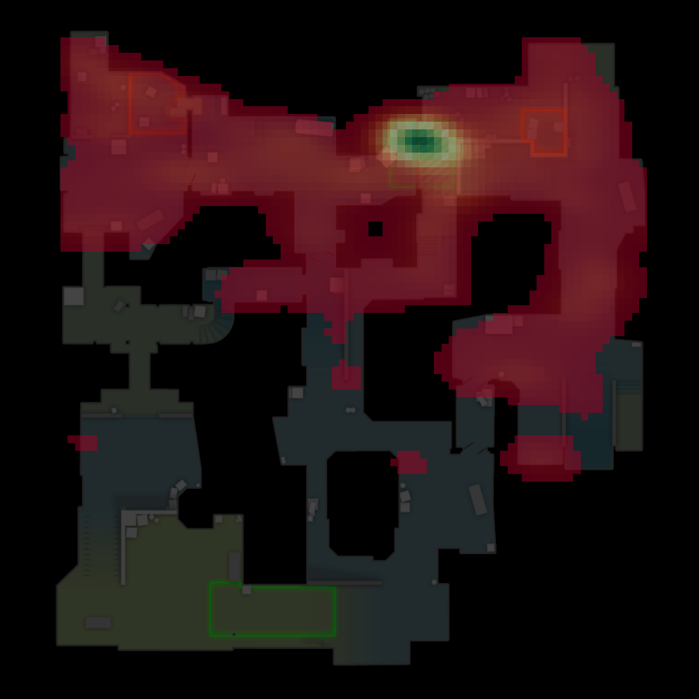
Heatmap

Finally, you can also create heatmaps. Below, we create heatmaps for a random sample of 100,000 player locations in the demo. The available method options are hex, hist and kde. You will also want to play with the size parameter. The values shown below are good starting points for the corresponding method, but it will depend on what you are visualizing.

[25]:

from awpy.plot import heatmap

player_locations = list(
    dem.ticks.filter(pl.col("health") > 0, pl.col("side") == "ct")[["X", "Y", "Z"]].sample(100000).iter_rows()
)
fig, ax = heatmap(map_name="de_dust2", points=player_locations, method="hex", size=20)

[27]:

from awpy.plot import heatmap

player_locations = list(
    dem.ticks.filter(pl.col("health") > 0, pl.col("side") == "ct")[["X", "Y", "Z"]].sample(100000).iter_rows()
)
fig, ax = heatmap(
    map_name="de_dust2",
    points=player_locations,
    method="kde",
    size=80,
    kde_lower_bound=0.01
)